
A data-centric approach to the study of system-level prognostics for cyber physical systems: application to safe UAV operations


Abstract
Maintaining safe operations in cyber physical systems is a complex task that must account for system degradation over time, since unexpected failures can result in the loss of life and property. Operational failures may be attributed to component degradation and disturbances in the environment that adversely impact system performance. Components in a CPS typically degrade at different rates, and, therefore, require continual monitoring to avoid unexpected failures. Moreover, the effects of multiple degrading components on system performance may be hard to predict. Developing and maintaining accurate physics-based system models can be expensive. Typically, it is infeasible to run a true system to failure, so researchers and practitioners have resorted to using data-driven techniques to better evaluate the effect of degrading components on overall system performance. However, sufficiently organized datasets of system operation are not readily available; the output of existing simulations is not organized to facilitate the use of data-driven machine learning techniques for prognostics. As a step toward addressing this problem, in this paper, we develop a data management framework and an end-to-end simulation testbed to generate such data. The framework facilitates the development and comparison of various system-level prognostics algorithms. We adopt a standard data-centered design methodology, combined with a model based engineering approach, to create a data management framework that address data integrity problems and facilitates the generation of reproducible results. We present an ontological design methodology centered around assets, processes, and data, and, as a proof of concept, develop an unmanned aerial vehicle (UAV) system operations database that captures operational data for UAVs with multiple degrading components operating in uncertain environments.
Aim: The purpose of this work is to provide a systematic approach to data generation, curation, and storage that supports studies in fault management and system-level prognostics for real-world and simulated operations. We use a data-driven simulation-based approach to enable reliable and reproducible studies in system-level prognostics. This is accomplished with a data management methodology that enforces constraints on data types and interfaces, and decouples various parts of the simulation to enable proper links with related metadata. The goal is to provide a framework that facilitates data analysis and the development of data-driven models for prognostics using machine learning methods. We discuss the importance of systematic data management framework to support data generation with a simulation environment that generates operational data. We describe a standard framework for data management in the context of run-to-failure simulations, and develop a database schema and an API in MATLAB® and Python to support system-level prognostics analyses.
Methods: A systematic approach to defining a data management framework for the study of prognostics applications is a central piece of this work. A second important contribution is the design of a Monte Carlo simulation environment to generate run to failure data for CPS with multiple degrading components. We adopt a bottom-up approach, starting with requirements and specifications, then move into functionality and constraints. With this framework, we use a Monte-Carlo simulation approach to generate data for developing and testing a variety of system-level prognostics algorithms.
Results: We have developed a data management framework that can handle high dimensional and complex data generated from real or simulated systems for the study of prognostics. In this paper, we show the advantages of a well-organized data management framework for tracking high-fidelity data with high confidence for complex, dynamic CPS. Such frameworks impose data logging discipline and facilitate downstream uses for developing and comparing different data-driven monitoring, diagnostics, and system-level prognostics algorithms.
Conclusions: In this paper, we demonstrate the design, development, and use of an asset, process, and data management framework for the research to develop prognostics & health management applications. This work helps fill a gap for system-level remaining useful life studies by providing a comprehensive simulation environment that can generate run to failure data, and a data management architecture that addresses the needs for system-level prognostics research. The framework is demonstrated with a Monte-Carlo simulation of a UAV system that operates multiple flights under different environmental conditions and degradation sources. This architecture for data management will enable researchers to conduct more complex experiments for a variety of cyber physical systems applications.
Keywords
INTRODUCTION
Cyber Physical Systems (CPS) are systems that integrate computing, networking, and physical processing and are comprised of one or more embedded computing platforms. They interact with the physical environment, and often times with humans. All physical systems degrade with use over time, and the added uncertainties in the environments these systems operate in (e.g., changing wind and weather conditions) makes it imperative to track system components and overall system performance. Prognostics and Health Management (PHM) can support the decision making required to facilitate safe flights; however, developing System-Level Prognostics (SLP) algorithms remains a challenging task due to the lack of real-world data or high quality simulation data. This is for two reasons: (1) it is not practical from a safety or cost perspective to run a real system to failure; and (2) currently available simulations do not utilize a standardized data management framework for the generation, organization, and storage of data.
In this paper, we develop a data management framework and data generation scheme to support data-driven approaches to SLP, which refer to approaches where system health and system Remaining Useful Life (RUL) are tied to overall system performance under realistic operating conditions. Our framework provides the context for developing data-driven machine learning models that support SLP and computation of system RUL. These approaches use a Monte-Carlo stochastic simulation to generate operational data for UAV systems with multiple degrading components flying a number of trajectories that are subjected to wind conditions that are modeled as stochastic processes. Our key contribution is a data management framework that facilitates the generation, curation, usage, and storage of simulation data that encompasses multiple operating and environmental conditions to facilitate studies with multiple machine learning algorithms for RUL and SLP analyses. We discuss below the motivating factors of this work, the challenges that we address, and our key contributions to the field.
Background & motivation
The use of UAVs has rapidly grown over the last few years across a wide variety of applications that include aerial photography, surveillance, package delivery, cartography, agriculture, and military missions. As adoption and use of these vehicles increase, so does the risk of failures during flight that can result in a loss of money, time, productivity, and most importantly, human lives. Components of these systems naturally degrade over time with continual use, and, consequently, the risk of failure during flight increases. The System-Wide Safety Project (SWS) (https://www.nasa.gov/aeroresearch/programs/aosp/sws), one of NASA's primary thrusts in the Urban Air Mobility (UAM) program, deals with all aspects of safety within the operational context of UAVs and is a driving force in this area of research.
System health management is critical for reliable and safe CPS operations. The inability to proactively manage system health can result in failures that lead to unnecessary down times, loss of assets, or even loss of human life. Therefore, researchers, practitioners, and system operators put a lot of effort into managing system health by monitoring the health of system components as well as overall system performance.
SLP contributes to the overall safety of operations by using estimation and prediction methods to improve system reliability and maintainability. A lot of work has been done on RUL estimation for individual components, but the literature that studies multiple component degradation and the effects on overall system performance is still sparse. The next generation of space and aerospace operations need to incorporate SLP methods for effective and safe operations.
NASA recently commissioned the National Academy of Sciences to conduct an in-depth study of the benefits and challenges of Advanced Air Mobility [1]. A key finding related to safety was that the current state of the art in simulation technology is not adequate. The report discusses the need for better tools to address both simulation and testing. In recent years, using a mix of tools and frameworks, along with custom software written in various languages, researchers around the world have developed prognostics applications with great results. Despite this progress, Li et al.[2] summarize quite succinctly,
"existing literature addresses aspects of PHM design methodology and provides PHM architecture formulations. However, a systematic methodology towards a consistent definition of PHM architectures, i.e., one that spans the conceptual and application level, has not been well established."
Software tools & simulation methods
The development of simulation-based and data-driven environments that have grown to a level of complexity where managing the generated data becomes a burdensome task fraught with errors. Therefore, it is imperative for system health management platforms to adopt a robust and well-defined framework that focuses on the data management aspects as much as the simulation. More than 10 years ago, Uckun et al.[3] highlighted the lack of standardization within the PHM community and critically pointed out that many PHM experiments lacked statistical rigor. While statistical evaluation methods for PHM applications have made significant advances, the PHM community still lacks a universally accepted research methodology using simulations and standard conventions for data quality and management. Developing new technology often starts with creating simulations and simulation testbeds. Typically, these simulations are developed "in-house", rely on specialized dependencies, are poorly documented, and are often difficult to replicate or extend. To overcome these problems, we propose a systematic approach to designing end-to-end simulation systems, and our key claim is that the simulation approach should be designed around the data first - not the other way around.
Modeling and simulation tools such as Simulink, LabVIEW, or Modelica are industry standards for a number of engineering applications. They also facilitate the generation and use of data. However, these tools do not enforce any policies or rules on how the generated data is managed. These are open-ended tools, meaning there is no framework to specify and implement such policies or interfaces, it is all left to the user. Given the skill-set disconnect between engineers or research scientists, the users of these tools, and the database engineers or the enterprise software developers who typically implement data schemas, the data management practices and implementations needed to facilitate experimentation often fall through the cracks.
Morris et al.[4] remark that a well-organized approach to planning and reporting simulation studies involves formally defining the purpose of the study, exhaustively enumerating all sources of data, the parameters that are being estimated, the methods used, and performance measures. While they focus on the field of medicine, their methodologies may be easily expanded to other domains of study. Typically what is seen in the literature is an overemphasis on the purpose of the study and methods used, with little attention given to properly documenting the component modeling or data these components generate. Simulink is the underlying software tool used for the simulation environment in this work; however, we provide all of the building blocks necessary to ensure simulation conformity and reduce the burden on the end user.
The NASA Diagnostics and Prognostics Group has developed the Prognostics Python Packages, prog_models [5] and prog_algs [6]. These are a collection of open-source research tools for developing prognostic models, simulating system degradation, performing prognostics, analyzing results, and developing new prognostic algorithms. The Prognostics Python Packages encapsulate design improvements over the previously released MATLAB Prognostics Libraries (PrognosticModels, PrognosticAlgorithms, and PrognosticMetrics) and C++ Generic Software Architecture for Prognostics (GSAP) [7]. The packages implement common functionality found in PHM applications (e.g., state estimation algorithms, predictors, sampling methods) and provide clear interfaces and tools for extending that functionality. NASA also had an effort to explore the challenges associated with a Service-Oriented Architecture (SOA) for Prognostics, called Prognostics As-A-Service (PaaS) [8]. This effort explored different architectures for PaaS, including structures for long-term data storage to enable outer-loop model optimization approaches.
While the Prognostics Python Packages and GSAP focus on implementing common functionality across PHM applications and enforce constraints on the physics-based models and composition of components within a system, it does not provide any systematic framework for the handling or storage of data. A running theme throughout this paper is the importance of understanding and addressing data concerns first, and then building the simulation software around those requirements. The data management framework proposed in this work does just that, and enables researchers to focus on their specific experiments with little upfront effort to incorporate the data schema into their work. This framework can also interoperate with any of the tools discussed above. Next we discuss data generation aspects in more detail.
Data generation & management
Over the last several years, there has been a rise in the use of deep learning methods in prognostics research to achieve results that were previously unobtainable. Nevertheless, as we have seen, there is a general lack of data management and attention to data provenance in these studies, which results in data that lacks appropriate descriptors, unverifiable origins, or any of the other several aforementioned issues presented previously that make replication or validation tasks hard to achieve. We argue that these issues persist due to the lack of data management standards and policies. The goal of data management is to produce "self-describing datasets"[9] such that scientists and practitioners can discover, use, and interpret the data across multiple experiments.
Oracle (https://www.oracle.com/database/what-is-data-management/) defines data management as the practice of collecting, keeping, and using data securely, efficiently, and cost-effectively. One thing not specifically mentioned in this definition is data organization, however, it can be inferred that the ability to use data efficiently implies some form of underlying organization. Microsoft (https://dynamics.microsoft.com/en-us/ai/customer-insights/what-is-a-data-management-platform-dmp/) defines data management as the collection, organization, and activation of data from various sources to put into a usable form. They define this in terms of a data management platform as a tool to facilitate data management, a critical piece that is missing in the scientific and engineering literature. This point is perhaps the biggest reason why such poor data management practices exist within the PHM community (not to remark on the acumen of our researchers, but simply the identification of a skill-set gap that exists).
TechTarget (https://searchdatamanagement.techtarget.com/definition/data-management) adds to the above by bringing accuracy into the picture, which can be interpreted as a form of assurance on the validity of the data and its provenance. Munappy et al.[10] define data management specifically for deep learning applications as a process that includes collecting, processing, analyzing, validating, storing, protecting, and monitoring data to ensure consistency, accuracy, and reliability of the data are intact.
However, these definitions do not address how this data is generated or its origins. This is one point of contention that must be addressed within the context of engineering or scientific disciplines that use simulation studies to draw conclusions. These studies are used to drive technological development of some system or algorithm that is eventually used in the real world, with real implications, and the validity of the data used is of utmost importance. Therefore, our definition includes data generation, in addition to the definition proposed by Munappy et al.[10], as follows:
Definition 1 (Data Management for CPS)A formal method for generating, validating, storing, documenting, and retrieving data that guarantee data security, consistency, availability, and persistence even long after the project that generated such data is finished.
Most of the effort in the application of machine learning algorithms is spent on data preparation[11]. The performance of a machine learning algorithm is directly related to the quality of the data sets employed for the learning task. Machine learning models are highly dependent on the underlying data, and, therefore, consistency, accuracy, and completeness of the data is essential to train models that are capable of sufficient generalization and performance[10]. Thus, good data management principles and practices need to be adopted throughout the entire development process. The majority of engineers focus on the development of the machine learning algorithms and simply deal with the fact that data preparation is going to be their most time-consuming part. This is largely because of the gap that exists between the skill-sets of a data management professional and that of a machine learning engineer.
Data consistency is hard to achieve or guarantee without a systematic and pragmatic approach to data management. Lack of consistency in the data ultimately results in a poorly trained model and has negative effects on any downstream processes[12]. Data validation can address these problems, and a properly implemented data schema can perform automatic validation, alleviating many of these issues. Lack of metadata or data descriptors creates confusion and poor understanding of the data, resulting in ambiguous data semantics that makes data discovery a cumbersome and sometimes impossible task. Data dependency, memory management, concurrency, the problem of noisy data, and data inconsistency can be solved in an integrated manner using a DataBase Management System (DBMS) within the workflow of simulation studies or machine learning applications [13].
Most datasets discussed in the literature are schema-free[14], meaning they do not share a standard format. This results in data organization methods that do not conform to a set of predefined rules or systems of organization. As a result, validating machine learning models is a major challenge. Accessing data from one dataset may not be the same as in another, even if the datasets are for similar applications. A well-defined data schema is necessary as it encodes and specifies what correct data is, and valid types and ranges for the data. In this manner, it enforces data relationships and other constraints to ensure data validity. Our aim is to propose a data schema that provides standards and explicit rules for data management for the PHM community to address the issues outlined in this paper. We provide this data schema and discuss the primary SLP use case next.
System-level prognostics
Prognostics brings together the study of how systems fail with life-cycle management to ensure safe and proper operations of the system [15]. Put simply, prognostics is predicting how a system's state and performance will change with time, and when a future event, typically End Of Life (EOL), or some safety or performance threshold violation[16], will occur. One common approach to assessing when failure will occur is to use empirical data provided by component manufacturers, such as Mean Time Between Failure (MTBF). However, MTBF specifications fail to account for system usage, therefore, are limited in their practical usability, especially when systems operate under a variety of operational and environmental conditions. Prognostics, in contrast, encompasses methods for estimating future performance based on telemetry data from system sensors, its current state of health, and predicted use over time. Because prognostics methods project system behavior into the future, the predictions are uncertain and are often expressed as probability distributions with confidence bounds [17].
In general, prognostics methodologies can be divided into three basic categories [18, 19]:
1. Data driven: These methods use probability-based [20] and machine learning algorithms [21] to map component measurements to the degradation parameters of a component, and often need run-to-failure datasets that are rarely available. Regression and deep learning techniques fall into this category.
2. Model based: This prognostic approach uses first principles physics and differential equation models of the system dynamics to develop parameterized degradation models of a component [22, 23]. Filtering techniques that utilize different Kalman and Particle Filtering techniques fall into this category.
3. Hybrid approaches: Hybrid approaches combine the best aspects of model-based and data-driven techniques. For example, Neerukatti et al.[24] proposed a hybrid approach for damage state prediction using a crack growth model and then showed using regression techniques how the model could be updated as new measurements became available. They demonstrated that the hybrid approach was more accurate and reliable than pure data- or model-based methods. This approach easily extends from the component level to the system level, where models of the components are used to update the component and state degradation parameters, and the generated data is used to make RUL estimates for individual components as well as the overall system.
Typically, prognostics is used at the component level to predict when an individual component, such as a battery or motor, will fail. This approach does not account for multiple degrading components in a system, and ignores the interactions between the individual components when estimating overall system health. SLP studies the combined effects of multiple degrading components in a system on overall system behavior and performance [25].
Definition 2 (System-Level Prognostics (SLP))SLP is a methodology for estimating future performance and time of events, such as component and system End of Life (EOL) or performance threshold violation, for
SLP must account for uncertainty, external influences, component damage accumulation, the interactions among these components, and the effects of multiple component degradation on system performance. Components interact with one another, so individual component degradation is no longer an isolated function of inputs and environment, but includes the complexities of interactions with other components. Degradation models that predict performance at the system level are an aggregation of the individual component degradation models, and because the interactions can be complex and nonlinear, they are not solvable analytically. In addition, variability in the environment parameters and uncertainty in the aggregated degradation functions necessitates the use of stochastic simulation methods to derive system performance over multiple missions. Events of interest in system-level prognostics include EOL for individual components (computed from RUL estimates) and system life (computed using estimated system performance). System EOL represents an estimated point in time when the system performance drops below pre-specified thresholds. System failure is expressed as the union of component failure conditions in conjunction with the violation of one or more system-level performance constraints. This is further discussed in sections 3 and 6.
In our previous work[26], we demonstrated that system performance degrades much faster than individual components due to the nonlinear effects of the joint interactions among the components and their degradation functions. However, we did not perform true RUL computations, and instead performed short-term forecasts via linear extrapolation, which only detected EOL events within the forecast horizon. This method also assumes that system-level performance degradation is linear within the forecast horizon, which may or may not always be guaranteed. While these predictions were accurate, they lacked a confidence interval because a Monte-Carlo base stochastic simulation was not used to account for uncertainty.
Perhaps the first true system-level prognostics approach that addresses these shortcomings with a convergent confidence interval with the use of Monte-Carlo simulations was demonstrated by Khorasgani et al.[25]. They developed a formal framework for SLP and applied it to the analysis of a full-wave rectifier circuit consisting of two capacitors concurrently degrading at different rates. The authors defined system-level RUL prediction as a function of the set of component degradation models, degradation parameters, system performance function, system performance threshold function, and the probability density functions of the system state variables. By combining the degradation rates of individual components using a particle filter approach, they generated accurate and stable results for system RUL events, i.e., when system performance dropped below pre-specified thresholds. We have incorporated this approach into the simulation environment developed in this paper and discuss it in greater detail in the following section.
There are a large number of excellent articles within the PHM literature that have led to health management advances that are being deployed today for real-world use-cases [27, 28]. However, many of these are application-specific methods, when viewed from a larger context of SLP are difficult to generalize across systems or applications [29, 30]. A large contributing factor to this is the increasing system complexity and the sheer volume of data generated from these systems. As system complexity continues to increase and physics-based models become more expensive to develop and maintain, more advanced data-driven machine learning techniques are required to support prognostics and health management methodologies and applications. This need paves the way for deep learning and reinforcement learning based prognostics, which require large amounts of data for training and validation. Such datasets simply do not exist, and for practical reasons, as outlined above, they must be generated by simulation. This leads to a set of primary challenges that we address in this paper.
Challenges
Very little real operational data is available for systems that are run to failure due to several reasons, primarily being that of safety and cost. Developing a simulation-based data repository for system-level prognostics to address this problem is a big challenge. On the one hand, simulation models are not an exact replica of the real system or how the system may operate in different environments. On the other hand, mathematical representations of system performance degradation are not easily derived, even when component degradation and system dynamics models are known. A number of run-to-failure experiments have been conducted for single components in isolation [31-33], but these experiments do not capture the nonlinear feedback loops among multiple components degrading simultaneously within a system, and the effects of their degradation on system performance. Only recently has a dataset been released that includes simultaneously degrading components [34], but the issues with standardized conventions around data management persist. In this paper, we address this issue and demonstrate the data management framework with a simulation that replicates realistic scenarios where multiple components of a complex system degrade during system operations.
A second challenge we address in this paper is to make the simulated data generation process transparent so the experiments can be replicated and results validated. Traditional methods for managing data from experiments employ predefined naming conventions and file hierarchies, with logs written during runtime as part of code execution. However, Almas et al.[12] explain that there is a critical need to describe and document more details of the properties of the component and system behavior data, as well as the relationships between the components, that cannot be done by writing files to disk. These details are captured in metadata, which needs to be made an explicit and integral part of documentation to ensure that the data descriptions are accurate, and validation exercises can be performed. Data generated from complex, multi-component simulations must ensure that robust data storing conventions are followed, which becomes a daunting task without a well-defined interface and data schema available. This is known as data provenance, and guarantees that the stored data conforms to predefined standards.
Contributions
The primary contribution of this work is a data management framework that allow for easy data processing of the generated data for a variety of applications. The data management framework imposes constraints on the generated data as well as the way the simulation is composed. This is accomplished with an asset-process-data paradigm, and is discussed in greater detail in the Methods section. Tracking the metadata and intricate relationships among all of the different data sources and types is essential to a robust data management framework. The retrieval, usage, and post-processing of data then becomes much more simplified and scalable, making the development of deep learning or reinforcement learning models much easier. The framework itself can interface with any type of system, real or simulated, and multiple systems can be tracked simultaneously. The framework can be used in production environments with real operational data feed coming from live systems, or with simulated environments where data is generated. We provide a stochastic simulation testbed in conjunction with the framework that allows for the seamless composition of component degradation models into a dynamic model that generate system performance data for complex cyber physical systems. Such an end-to-end simulation framework supports the data generation process. Overall, this allows for (1) a more comprehensive study of degradation, failure, and RUL; (2) the generation of curated datasets that make it easier to run machine learning experiments to support SLP and RUL studies; and (3) flexibility to simulate a multitude of systems under varying environmental and operational conditions.
METHODS
This work brings together simulation methods and data management practices into a unified framework to support data generation experiments for developing data-driven models for system-level prognostics. We formalize SLP, building on Definition 2, and discuss the implementation of the simulation environment. We then show how the data management framework integrates with this simulation environment to organize and store the data for future use.
System-level prognostics
The goal of system-level prognostics (definition 2) is to predict the RUL of a system considering the interactions among its different components and the effect of degradation over time on system performance. System failure is attributed to individual degrading components in the system and the effect of multiple degrading components on overall system performance. Therefore, system EOL is a result of physical failures attributed to the effects of multiple component degradation, and the operational failures that result from the loss of system performance with respect to a set of predefined performance constraints (e.g., maintain system trajectory deviations to
The system
where
which is the earliest point in time when a system performance parameter threshold is violated. The system performance threshold function
where
The set of constraints is defined to account for both component and system-level performance metrics, and they are computed based on states
Definition 3 (System degradation model)The system degradation model is defined as
where
The noise and disturbance parameters,
System-level data generation for prognostics
Individual component behavior depends on many factors, including usage and the health and functionality of other components. The system behavior is typically a function of the behaviors of these tightly coupled components, which results in complex nonlinear dynamics. All of these phenomena need to be accurately captured in the system model. Therefore, the system dynamic function
The study of reliable system-level prognostics methodologies is critical for safe operations of complex cyber physical systems. Currently, this is a very active area of research [35]. Due to the challenges in developing prognostics applications discussed in the previous sections, we have proposed a data management framework to support prognostics studies for real or simulated systems. All cyber physical systems are made up of multiple components and subsystems, and each of these components degrades with use and over time. By measuring system inputs and outputs over time, we can track the degradation and performance of individual components, as well as the overall system. Therefore, the set of relevant input and output variables in the system as well as the parameters associated with components and system performance, constitute the data management framework, as illustrated in Figure 1.
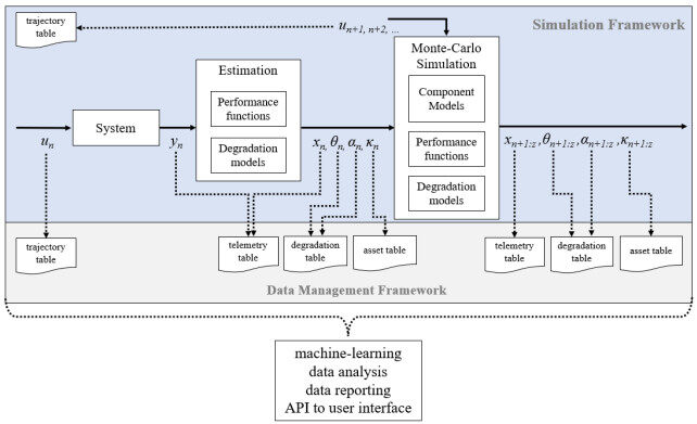
Figure 1. System-level data generation for prognostics applications. The decoupling of the data generation, whether it is from a real system or a simulation, from data organization and consumption (machine-learning, data analysis, etc.), allows for multiple systems and system types to be studied with the same core functionality and codebase.
Simulation approach
We utilize a Monte Carlo (MC) approach as the basis for a stochastic simulation framework to generate system-level data given a set of component, environmental, and degradation models; a series of inputs; as well as performance threshold functions. Stochastic simulation accounts for the different forms of uncertainty within the environment, degradation models, and state-space estimates. It should be noted, however, that the data management framework is designed to work with real systems as well as simulations. Therefore, one does not need to employ a specific simulation system to use the data management framework if a real system is available. For PHM applications, however, run-to-failure data needed to develop prognostics algorithms, is not easily available since it is uneconomical or even hazardous to run a real system to failure. Therefore, accurate simulation systems are the feasible recourse for systematic studies of system-level prognostics. Our simulation environment implements a set of MATLAB® scripts that run in parallel to take advantage of multi-core CPU architectures without requiring any specialized parallelization computing libraries. We describe the simulation architecture in parts to facilitate a better understanding of how the individual pieces work together, and begin with the data sources for the simulation.
The torque-load relationship model was derived via polynomial fitting of test data obtained from a publicly available dataset. The aerodynamics, DC motor, and continuous battery models were adapted from previous publications [26, 36-39]. The battery degradation model came from test data obtained from NASA's data repository. Motor degradation models were developed by experimentation using reasonable assumptions on how long the motors are expected to last based on manufacturers' datasheets. Wind gust models for typical urban environments were generated by studying the literature [40]. The stochastic simulation of the UAV system and environment uses input/model data from several different sources, shown below in Table 1.
Data sources for stochastic simulation
The simulation framework is executed in two parts that repeat until EOL is reached. First is the true system simulation, a facsimile of a real system, followed by the Monte-Carlo stochastic simulation, which generates the necessary degradation data for prognostics analyses. The Monte-Carlo simulation is designed to run 24 parallel systems until system EOL is reached for all 24. Afterward, the true system is simulated again for the next mission. This process repeats until the true system reaches EOL, at which time the data collection process is complete. This is depicted in Figure 2. This Monte Carlo simulation process and the data management framework can be applied to any CPS. In this paper, we demonstrate its application to a UAV system.
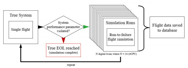
Figure 2. Stochastic simulation framework for data generation.
A single flight flow diagram is shown in Figure 3. First, the workspace is initialized by connecting to the database and loading information such as available trajectories, system performance thresholds, and initial conditions (For a complete description and documented example code in Matlab, see https://github.com/darrahts/uavTestbed/blob/main/livescripts/example.mlx). Other simulation parameters, such as the controller gains for the PID controllers, are also specified. This data is stored in the base workspace of the calling process, where parallel processes have their own information and do not share data. Next, an existing UAV model is loaded from the database or a new UAV model is created. If multiple UAVs are part of the SLP study, one can be selected by serial number or ID. Then, a trajectory is assigned to the selected UAV in one of several ways, with a random selection from a set of predefined trajectories being the default method. Alternatively, a flight plan can be specified as a set of valid waypoints (a waypoint and an obstacle cannot have the same coordinates).
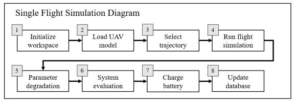
Figure 3. Single flight simulation.
The flight is then simulated and all of the flight variables and parameters (especially the degradation parameters associated with components) are recorded along the flight path. After flight termination, the degradation parameters for the UAV model are updated and the system performance parameters are evaluated. The flight can either end successfully, or end with a stop code (i.e., a performance parameter violation), and this information is logged. At the end of every simulation run (i.e., a mission), the battery is recharged. Charging cycles also add to battery degradation, just as the battery discharging process, but the rates of degradation for these two processes are typically not the same. This is captured by a parameter whose value ranges between 1 (same effect as discharging) and 0 (no effect). In this work, it is set to 0.75. The asset use and flight data are also recorded in the database.
System description
The system used in our experiments is a generic octorotor UAV using parameter values provided in [36]. Table 2 lists the variables and their descriptions. The Newton-Euler equations of motion for a rigid body dictate the dynamic behavior of the system as follows[38]:
Dynamical variables of the system
| Variable | Description |
| Force applied to body frame | |
| Force generated by the motors | |
| Drag force | |
| Angular velocity of the | |
| Angular acceleration of | |
| Current demand from | |
| Input voltage to the motors | |
| Total current demand from entire system | |
| Internal diffusion current | |
| Hysteresis voltage | |
| Output voltage | |
| Open circuit voltage | |
| Sign of current | |
| Battery state of charge |
where
The octocopter made up of multiple components, which simultaneously affect the overall system performance. For example, the degradation of a motor affects the resulting generated forces and moments (
where
The airframe, motor, and battery parameters and their values are given in Tables 3, 4, and 5, respectively, shown below. Together, these values are used in the simulation environment to create the physics-based models that are simulated to generate data for usage in downstream processes such as those shown at the bottom of Figure 1.
Airframe parameters
| Parameter | Desc | Value |
| Mass | Total mass | 10.66kg |
| Inertia matrix | ||
| Cross sectional area | ||
| Arm length | 0.635m |
Motor Parameters
| Parameter | Description | Value |
| *degradation parameter | ||
| Equivalent motor resistance | ||
| Back EMF | ||
| Friction torque | ||
| Viscous dampening | ||
| Inertia | ||
| Rotor thrust coef. | ||
| Rotor drag coef. | ||
| Translational drag coef. | ||
Battery Parameters
| Parameter | Description | Value |
| *degradation parameter | ||
| Total charge capacity | ||
| Coulombic efficiency | ||
| Voltage decay constant | ||
| Polarization constant | ||
| Polarization constant | ||
| Warburg impedance | ||
| Internal resistance | ||
| Diffusion resistance | ||
| Initial voltage | ||
System model
The five major blocks of the system-environment simulation are navigation, control, powertrain, dynamics, and environment as depicted in Figure 4. Initially, values for position and velocity are provided in the UAV's start state in a continuous space 3-D world. A reference trajectory is derived offline before flight and supplies the navigation block with coordinates to fly to. The GPS model adds position and velocity noise (with a bias of 0 as we are not modeling sensor faults) and supplies the control block with the reference position, true position, true velocity, GPS position, and GPS velocity. The control block calculates the position errors and uses PD controllers for orientation and angular velocity. It outputs an N-dimensional array of voltage reference signals; in the case of an octorotor, N = 8.
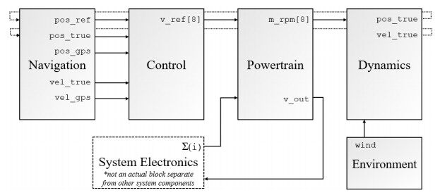
Figure 4. Simulation model.
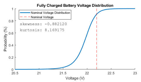
Figure 5. Nominal voltage distribution.
The voltage reference signals are fed to the powertrain block, which contain the motors and battery models. The second input to the powertrain block is the current demand from all other components in the system (such as the GPS). The output of the powertrain block is a vector of motor RPMs that is sent to the dynamics block, which implements the aerodynamic equations of the UAV. The environment block is also an input to the dynamics block, where external factors such as wind gusts are translated to forces that are applied to the airframe. The output of the airframe block is updated position and velocity in the inertial axis, which is sent to the navigation block, and the flight control process is repeated.
It is important to also discuss the sources of uncertainty and noise, as well as the random variables in the simulation. Noise is attributed to processes and measurements within the system, system components, and environment. Measurement noise for a given parameter is modeled as an additive value. Uncertainty is modeled similarly and is captured in the confidence intervals for a given random variable, such as for the component degradation models. For each degradation parameter,
Another source of uncertainty is the variation in the fully charged battery voltage for each charging episode. This is modeled as a skewed distribution in Figure 5 with approximately 90% of the values falling between 21.2 and the nominal voltage, 22.2, and 10% of the values falling between 22.2 and 22.6. This effectively models what is experienced in the real world for charging batteries: sometimes they overcharge or undercharge, and usually the final charge value is within some range of the rated output voltage value.
System performance parameters
System-level performance parameters are random variables computed from system variables, and they are a proxy for the State Of Health (SOH) of the system. For the UAV, overall system performance is a function of the SOH of the battery and the SOH of the eight motors. A Sigma Point Kalman Filter [47] is used to perform battery (state and degradation) parameters estimation, and resistance measurements with additive noise are used to assess the motor (degradation) parameter. These are common and well-documented methods not discussed further in this work. We instead will focus on the implementation of the system-level performance parameters.
The first two parameters are (1) the battery State of Charge (SOC) (
System performance parameters
| Parameter | Name | Description | Value |
| Battery state of charge | Impacts flight time and load capacity | 20% | |
| Battery output voltage | Impacts flight time and load capacity | 18.71v | |
| Average position error | Impacts risk of collision | 2.8m | |
| Position error standard deviation | Impacts risk of collision | .7m |
The set of system performance parameter constraint functions (
Definition 4
The battery state of charge shall always remain above 20%.
The battery output voltage shall always be greater than 18.71 volts.
The average position error shall always remain below 2.8 meters.
The position error standard deviation shall always be less than.7 meters.
Degradation models and environment conditions
In this work, we consider the effects of the simultaneous degradation of eight motors and the battery pack. Specifically, stochastic degradation profiles are generated for three parameters: the equivalent electric resistance of the motor coils (
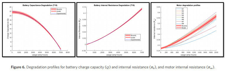
Figure 6. Degradation profiles for battery charge capacity (
The battery charge capacity is the amount of charge available in a fully charged battery. Battery charge capacity degrades as the battery undergoes multiple charge-discharge cycles over time. This can be attributed to the internal chemical processes within the battery as well as environmental factors, such as temperature. The degradation rate for
Besides simultaneous component degradation, environmental factors can affect the operation and performance of the system. In this work, we consider three environmental parameters: temperature, wind, and obstacles. Temperature is known to have an effect on both flight and battery performance. At high temperatures, flight performance is reduced due to the aerodynamic affects of increased molecular air speed causing a reduction in lift. This reduction in lift causes the motors to draw more current to produce the increased forces necessary to counter the reduction in lift. This further increases the rate of damage accumulation for the motors and the battery. Furthermore, in [52], the authors show that battery aging increases in high temperature conditions, and battery charge capacitance decreases in low temperature conditions.
Wang et al.[53] provide a comprehensive analysis of different types of wind conditions and describe models of their effects on flight. Wind effects create load on the airframe, which puts stress on both the motors and the battery as the controller works to compensate for this additional force to maintain stability. While many different wind models exist, we implement a discrete wind gust model that acts along the three axes of UAV flight. Each axis samples a magnitude and direction from a normal and uniform distribution, respectively. Then, a duration value is sampled from a distribution where
Obstacles are either static, i.e., their location in the global coordinate frame (time and space) does not change, or they are dynamic, in which case their temporal-spatial location changes. Static obstacle influence system behavior during the trajectory planning phase and are easier to deal with than dynamic obstacles. In this experiment, we consider static obstacles that are part of the map, and save dynamic obstacles for future experiments.
Trajectories
The flight trajectory of the UAV (see Figure 7) plays a role in its overall safety and risk of failure during flight. Trajectories with sharp movements can also impose heavier impulse loads on components, which as discussed above, impact degradation rates. To study these effects in depth, the trajectories must be tracked and linked to other data objects. In general, a trajectory is represented as a multidimensional array capturing a time series, where each axis ([0,1,2]) is the equivalent x, y, z axis in space. A triplet is a single slice across the matrix that represents a specific point in space where the UAV is located at a specific time. Trajectories can be grouped into sets based on distance, estimated flight time, risk, or reward (although risk and reward are not considered in this work). Six trajectories of the set of trajectories flown (eight in total) are shown in Figure 7. Trajectories are formed in two steps using probabilistic roadmaps (PRM), followed by B-spline smoothing (see https://github.com/darrahts/uavTestbed/blob/main/livescripts/trajectories.mlx for a Matlab implemention of generating trajectories.) described below.
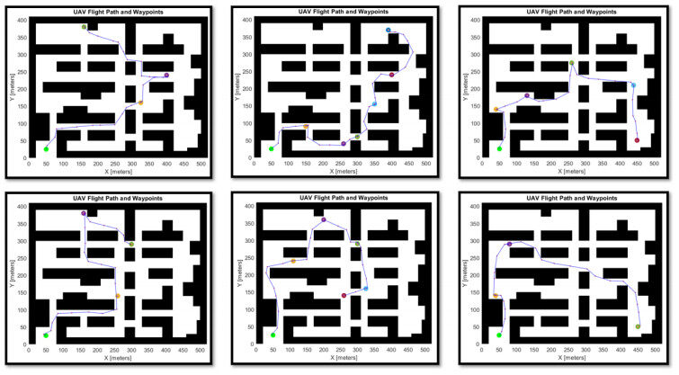
Figure 7. Available Trajectories in set
A Probabilistic Roadmap (PRM) is a graph structure where the nodes represent collision-free waypoints and the edges represent a realizable path between these waypoints ([54]). Two parameters, number of nodes and maximum connection distance, must be supplied by the user. First, the graph is created by generating random nodes in the search space, and then checking if they are valid nodes. Then, each node is connected to every other node within the maximum connection distance, so long as that connection is also valid using the k-nearest neighbors method. Generating a graph is the first phase of the algorithm, which is executed offline based on the navigation map. In the query phase, the start location, waypoints, and end location are connected to their closest nodes of the graph, and the path is obtained by using Dijkstra's shortest path algorithm. If there is no valid path (i.e., collision-free) from a supplied location to an existing node on the graph, then that location is deemed unreachable. Figure 8 depicts three scenarios of the trajectory generation process that show the outcome of different parameter selections.
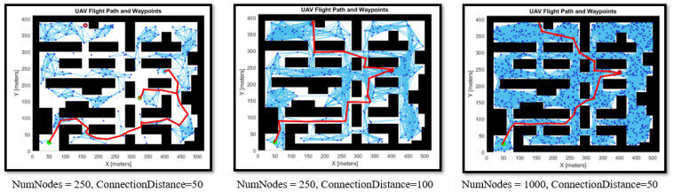
Figure 8. Trajectory generation. (L) too few nodes have been supplied and the waypoint at (160, 390) cannot be reached. (M) the connection distance is increased but now it is clear that the flight path is not optimal. (R) enough nodes have been selected and the connection distance has been reduced, providing the optimal trajectory.
Piecewise B-spline curves of degree
Monte carlo simulation
A Monte Carlo simulation approach is used to derive data-driven models and provide confidence bounds on what is being estimated, in this case, the system-level RUL. This is in the context of its safety goals discussed above, as well as operational goals, such as flying to each waypoint in the trajectory. Algorithm 1 presents the pseudocode for the Monte Carlo simulation program, and is detailed below.
Algorithm 1: Monte-Carlo System-Level RUL Data Generation Simulation Process Result: System-Level RUL Distribution
Data: models
Input:
Output:
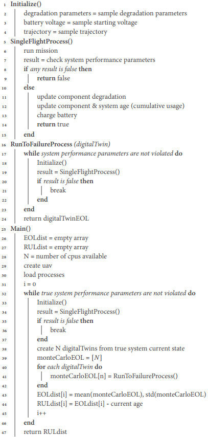
The algorithm consists of three functions in addition to Main, which are Initialize (line 1), SingleFlightProcess (line 5), and RunToFailureProcess (line 16). This organization makes the code more readable, and allows the reader to refer back to Figures 2 and 3, which depict the simulation program graphically. Starting in the Main function on line 25, two empty arrays are instantiated that hold the EOL and RUL distribution values at each iteration. The value
In line 30, degradation processes are attached to the UAV simulation, which means that the tracking mechanism that works behind the scenes can inform researchers of the degradation models that were used for this experiment. In line 33 (Initialize), the degradation parameter distributions are first estimated, and then sampled to produce
Line 7 of the SingleFlightProcess is where the system performance parameters are checked, which refers back to Equation 3 in Section 3. After each flight of the true system and subsequent steps in the single flight process, the program enters the Monte Carlo block in lines 38-44 (Figure 3, Section 4). A number of MC samples are created until a system performance threshold is violated by checking
In this current form, we allow the true system to reach actual failure as the stopping condition for the program, since this is a data collection experiment. In all other cases, the stopping criteria would be another boolean LTL function that operates on the most recent RUL distribution estimate. At the end of the program, a 2D array is returned, with the first dimension being the mean RUL, and the second dimension being the standard deviation.
Data management framework
Data sets that lack an organizational structure do not provide effective support for health management applications. Useful data sets that support PHM analyses must conform to explicit rules for data creation, storage, retrieval, and update. They also need to include Persistent and Unique IDentifiers (PIDs/UIDs) for data assets. Data curation can become a tedious and error prone task in the absence of a properly designed Extract, Transform, Load (ETL) pipeline. To address these concerns, we adopt an object oriented design methodology and bring together intersecting concepts from enterprise software development, data management, and engineering experimental design to establish our data management framework. We begin by outlining the key requirements and specifications of the framework, followed by an in-depth discussion of the key attributes and features.
Requirements
Design decisions are driven by requirements, which are themselves driven by higher level goals. In this case, the goal is to simplify and facilitate system health management analyses, and in particular, SLP research. We have developed four general and five specific requirements to meet this goal, as outlined below.
R1 - Reproducibility. This represents the ability to reproduce experiments, and, therefore, supports a better peer-review process while establishing connections with other experiments. This is accomplished by explicitly specifying data, meta data, and asset organization. This is also an important requirement for validation tasks.
R2 - Explainability. This is directed towards making the specific methodologies employed for tracking all of the influences explicit and transparent, from modeling approaches to algorithms used in the simulation and data generation process. Explainability is required to achieve proper data provenance.
R3 - Extensibility. The code base needs to be developed using a modular, decoupled approach behind well-defined interfaces that facilitate superficial changes and the running of new experiments without having to make substantial alterations to the underlying codebase or having to rewrite significant amounts of code. This makes it easier for engineers not familiar with data management practices to incorporate the framework into their experimental approaches. Overall, it supports wider adoption.
R4 - Maintainability. This is focused on ensuring that the codebase and data storage is consistent across multiple experiments. Maintainable systems also make it easier to track bugs and fix errors. Maintaining a consistent and modular code base makes it easier to run machine learning experiments that generate consistent and reproducible results. We do not deal with the software aspects of PHM applications (e.g., see the GSAP framework[7]), but these concepts apply to data management, and this requires the specification of a well-defined data schema.
R5 - System Composition. The framework should enable seamless composition of component and degradation models to construct the desired system models for simulation. This enables running a variety of prognostic experiments by pulling component and degradation models from a system library, instead of building models from scratch or trying to embed them in the executable code for every experiment.
R6 - Operational Variability. The framework should support multiple operational cycles, where a cycle is a single run of the system. Operational cycles are defined by assigning values to a set of parameters, such as the load setting for the charge-discharge cycle for a battery, and setting the waypoints to define an aircraft flight trajectory, or a sequence of deliveries for a UAV.
R7 - Monte Carlo Simulations. Monte Carlo simulations represent a generalizable approach to generating data associated with a problem specification, taking into consideration variations in operating and environmental conditions, which are represented as stochastic variables. They provide a systematic methodology for generating large amounts of data that support data-driven analyses.
R8 - Data Validation. Automatic validation of the data is a key requirement that ensures the data conforms to explicit constraints and can be guaranteed to be correct, without overburdening the user. This allows researchers to focus more on their specific application, and less on the nuances of ensuring the data is correct.
R9 - Data Integrity and Availability. The framework should also guarantee accessibility, discoverability, and persistence of data. This should be accomplished with an application programming interface (API) that exposes various methods for storing, retrieving, and updating records (among other functions).
A system designed to meet these requirements will allow for automated or semi-automated workflows that are self-documenting in terms of the data, meta data, and data provenance. Such a design pattern for data management within the context of PHM will improve the development pace and collaboration among researchers. Our data management framework adopts an asset, process, and data methodology to address these requirements. This framework captures and organizes high fidelity simulation data to support the development, testing, and evaluation of health management applications.
Framework design specifications
We have established six primary specifications to meet the above requirements in this framework. We provide a complete simulation environment for a UAV as reference implementation of this framework in MATLAB® and Simulink® (A complete simulation package that can serve as a stand alone application or as an example to build one using this framework can be found at https://github.com/darrahts/uavTestbed). The overall framework specifications are as follows.
S1. The framework shall be comprised of three primary parts - (1) assets, (2) processes, and (3) data. Assets are the tangible components that make up the system under study, in our case UAVs. Processes are time-dependent functions that represent internal or external influences that act upon the UAV. Data is any real value with meaning that is generated by an asset or process. This decomposition will become clear in the respective subsections that follow. A high level diagram that depicts these relationships is shown in Figure 9.
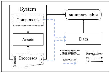
Figure 9. Abstract framework diagram.
S2. The data schema shall define the data type and validity constraints, and be implemented as a set of table definitions that enforce these constraints. This alleviates a substantial burden for researchers, the users of the data, by abstracting many low-level data operations common to many different kinds of experiments behind an application programming interface (API).
S3. For generality, we develop APIs in both Python and MATLAB®, allowing for use and integration among a wider group of researchers. There are already a substantial amount of innovative projects and experiments with UAVs using these two languages and an API in both languages will support wider adoption.
S4. Users shall be authenticated before access to the data is granted to ensure data security and integrity. Other users (such as a guest) might only be given "read only" access. Certain data fields automatically populate themselves based on default values or the logged-in user.
S5. The "delete" operation shall have no effect on any record. This is to ensure data persistence. Since the data generated is assumed to be inherently valid and accurate (via constraint checking at the database), every data record has meaning of some form. If there was a mistake in the simulation, the manifestation of that mistake is captured in the resultant data and should nonetheless be treated as "valid".
S6. The data schema shall be implemented using a relational database management system (RDBMS) with support on Windows, Linux, and Mac. An example is PostgreSQL (often referred to as simply Postgres), which is free and open source. Other RDBMSs may be used (such as MS SQL Server or MySQL), however, Postgres is a true open-source RDBMS that offers extensions and 3rd party integration, which have seen a large degree of success in the world of enterprise data management.
A system is comprised of assets, which are abstractions of user defined components. Assets can be affected by processes, which themselves can be internal (degradation via damage accumulation) or external (environmental influences). Processes can also have a transient effect on the overall system (i.e., wind gusts for a UAV). Together, components and processes generate data that is linked to the system and other information pertaining to the usage of that system via the summary table. All usage-based data tables link to the summary table, which in turn links to the system, the assets installed on the system, and the processes affecting the system at that time. A system can undergo multiple component changes and these changes are reflected in the underlying data automatically.
We now proceed to expand this high-level framework to provide more descriptions of the components, and how they interact to achieve the requirements.
Assets
Assets are the tangible components that make up a system, in our example, the system is a UAV, and the assets are the UAV itself and its components, i.e., the battery, motors, airframe, and a GPS sensor. Each asset acts as a first class object, meaning it is the archetype model that all components of the UAV inherit from. This includes many other types of components not listed above that may make up the UAV. All physical components are assets, including the UAV. This is perhaps one of the most fundamental concepts of the framework and central to interoperability among components, systems, environmental effects, and degradation models.
All assets have an associated asset-type (with predefined asset-types given in Table 7), which holds meta-data about the asset. The table name is
Asset-types
| id | Type | Subtype | Description |
| 1 | airframe | octorotor | osmic_2016 |
| 2 | battery | discrete_eqc | plett_2015 |
| 3 | motor | dc | generic |
| 4 | sensor | gps | generic |
| 5 | uav | - | - |
An asset-type must exist before an asset of that type can be created. This is stored in a table called
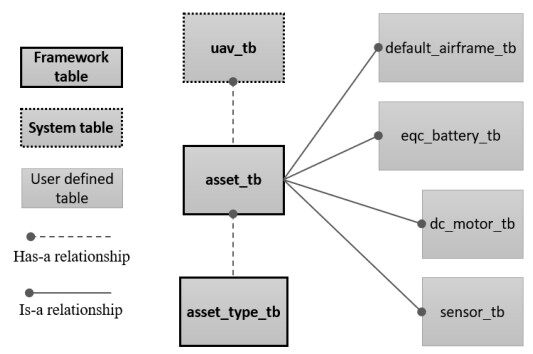
Figure 10. Relation diagram (assets).
Four other tables are depicted in Figure 10 that store the model parameters for the asset-types listed in Table 7. These are parameters of the component models and are specifically related to that component model type, a.k.a., asset-_type. There is a one-to-one relationship between a given model class and an entry in the asset-type table, however, there can be any number of model instances of the same model class. This is reflected in the real world, especially thinking about organizations that operate fleets of the same vehicle made of the same parts. Enforcing this constraint (and others) using a database management system is straightforward and works reliably when properly implemented. All other tables that have a relation with the asset table are defined with a data schema using the same mixed approach as described for the asset table. We direct the reader to the documentation (https://github.com/darrahts/phm_data_framework) for more in depth information on all aspects of the data schema and implementation. Each table (with the exception of
Processes
Processes capture dynamic interactions between the system and the environment. Many different types of processes can be modeled. In this work, we model internal component degradations and external wind gusts. Each component has its own set of degradation profiles and failure modes that are separate from, but affect the overall operation and health of the system. Therefore, the framework must have the ability to track processes just like tracking components. In a similar manner to modelling components as assets having asset-types, the process archetype also has process types (Table 8). Processes and assets are closely related as depicted in Figure 11. It is required that every process modeled be mapped to an asset, so as to track the relations between processes and components. This is something that is easy to lose sight of, and something as simple as a small parameter value change can have large differences in the resultant data. Therefore, processes and assets are tracked together. Each process has a foreign key relation
Process type table
| id | type | subtype1 | subtype2 | asset_type_id |
| 1 | Degradation | Battery | Capacitance | 3 |
| 2 | Degradation | Battery | Internal resistance | 3 |
| 3 | Degradation | Motor | Internal resistance | 2 |
| 4 | Environment | Wind | Gust | 1 |
| 5 | Environment | Wind | Constant | 1 |
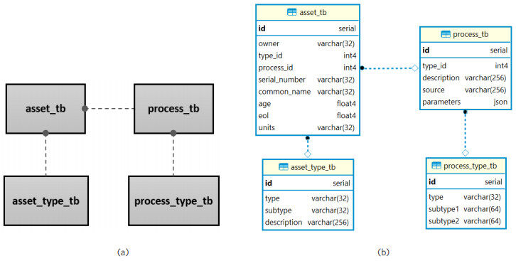
Figure 11. (a) entity relationship among processes and assets; (b) entity relationship with data fields and types.
Having a well-defined foundation for managing assets also makes parallelization and performing Monte Carlo simulations easier. Multiple assets can be created to run the same code in separate instances, separate machines, or even in the cloud. Data-driven experiments, this one included, are typically based on stochastic simulations and this flexibility simplifies planning, optimizing, and executing them. "The devil is in the details", and correctly storing and extracting data generated from these experiments can be very tedious and prone to errors. This framework addresses these challenges simply through its inherent organization and use of an underlying database management system.
Data management
We are especially concerned with components, degradation models, environmental models, and other internal and external events that generate information useful for prognostics applications. Metadata is just as important to capture as the raw data as well. Ensuring these complex interactions are captured and all relevant metadata and data from components, processes, the environment, and all other sources is the cornerstone of any data-driven CPS process, especially that of system-level prognostics. All data that is generated is inherently organized correctly when this framework is used in conjunction with a simulation environment. In this manner the entire process of data generation, storage, retrieval, and analysis among flights with different components can be executed with the same code. It is left to the individual practitioner to implement the dynamical models of their system; this framework handles everything else.
The data relationship diagram is shown in Figure 12, where three primary types of data are considered: degradation data, summary data, and telemetry data. The
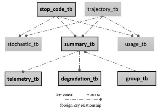
Figure 12. Relationship diagram (data).
RESULTS
The major challenges with run-to-failure data generation and data management were discussed in detail in Section 1. In this work, we demonstrate the use of a data management framework with a Monte-Carlo simulation of a UAV in an urban environment and by using the framework, we were successful in addressing all of the challenges discussed earlier. This includes the amount of data generated and complex inter-relationships among different data sources, as well as ensuring that we correctly interpreted the saved data from the experiments. Another key issue was needing the ability to experiment with different models without having to rewrite code, or deal with hard-coded model parameters. The framework handles all of these intricate details behind the scenes, and we highlight below how this framework can be used in any simulation environment using Python.
A primary example we highlight is the creation of asset types and assets. System component models are easily declared and composed using the API with a couple of lines of code as shown below. In line 1, the asset-type is created and returned as a dataframe, but if the asset-type already exists, it is simply returned. In line 2, the asset itself is created with the minimal number of parameters required (other options can be declared). Required parameters include the
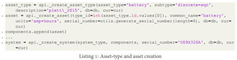
This is also completely decoupled from the model definition and implementation, and is what allows for different models to be used or composed into different systems. When an asset is created, a table in the database is automatically created using the
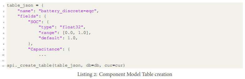
or the fields can be added individually.

These are just a few short examples of how the data management framework simplifies the creation of components, and allows the different data sources to be properly connected without any effort by the end user.
We discuss a few issues in relation to the experiment and data interpretation. System EOL is defined as the time one or more of the system performance thresholds are violated. This means that system EOL will take on different meanings, with different implications, depending on which performance parameter threshold is violated. Table 9 depicts the stop-codes for each flight in the study. The "true count" column represents each flight of the true system, from the first flight to the final flight (and 2 additional flights for verification). We can see from these results that the true system violated a performance threshold after 70 cycles (flights). The "stochastic count" column represents the final flight of each run-to-failure trace of all the Monte-Carlo simulation samples in the study. We can see the failure codes relate to battery performance and not controllability. One might then surmise that this UAV might still be capable of flying short trajectories. We considered a set of trajectories, each with similar characteristics in estimated load, distance, and duration. This implies that there may be another set of trajectories with different characteristics that the UAV could still fly. If the stop codes were related to position error, one might conclude that the individual properties of the trajectory are irrelevant, and it is not safe to fly at all. Such conclusions will ultimately rest with the policies and standards established by the organization conducting the flights. The data management framework provides a simplified and robust manner for storing, retrieving, and interpreting this type of data.
Stop codes for each true system flight and digital twins
| id | Description | True count | Stochastic count |
| *validation flights after EOL detected | |||
| 1 | Low soc | 0 | 1069 |
| 2 | Low voltage | 2* | 2131 |
| 3 | Position error | 0 | 0 |
| 4 | Arrival success | 70 | 0 |
| 5 | Average position error | 0 | 0 |
| 6 | Low soh (battery) | 0 | 0 |
A total of eight different trajectories were used in this work (6 are depicted in Figure 7) and a histogram of trajectory selection is shown below in Figure 13. The numbers at the top of each bar are the number of run-to-failure simulations conducted for that trajectory.
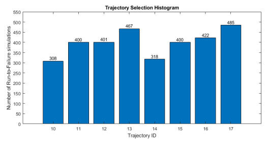
Figure 13. Trajectory selection histogram of the Monte Carlo simulations.
High-quality data is generated by ensuring the environment and degradation models propagate component-level health into system-level behavior. Metadata from the UAV components, environment, and data models are automatically recorded. The organization of the data imposed by the asset-process-data paradigm ensures it can easily be used to evaluate PHM applications and research questions.
DISCUSSION
In this paper, an asset, process, and data management framework for the research and development of PHM applications has been proposed. This work is motivated by the lack of comprehensive simulation environments and data management architectures that address requirements specific to PHM research, notably run-to-failure datasets and data organization schemes. From these requirements (among others), a set of specifications and rules were developed from which the framework was developed. The framework was demonstrated with an end-to-end simulation environment implemented in MATLAB®.
The lack of real-world system run-to-failure system data made it necessary to run simulation experiments. Closing the gap between real-world and simulation data can be facilitated through the use of the framework and methodology we have presented in this paper. The framework was designed to ensure that it can seamlessly work with real systems or simulations of systems, and the data will conform to the exact same standards. This will allow researchers to better understand their models when compared with real systems. Furthermore, the framework can support multiple systems simultaneously, regardless of the system type. Entire fleets of UAVs (or groups of any systems for the matter) can be studied for a wide variety of topics.
After initial experiments to validate the framework were successful, we conducted the system-level RUL experiment presented in this paper. This has led to additional questions that can be addressed through future work in this line of research. For example, in our experiments, we did not notice any significant effects of motor degradation because the battery always failed first, and this may be expected in the real world. How do these results differ if, instead of concluding that system EOL is reached based on operational requirements (such as flying trajectories of a certain class), we provide a different set of trajectories with less usage and shorter flight duration? Or, what if the battery was changed instead of stopping the experiment? How many battery changes will it take to notice the effects of motor degradation? How does the position error evolve over time after multiple battery changes and continuous motor degradation? How would system-level RUL be affected by different wind conditions or temperatures? What if we use different degradation models, or incorporated abrupt faults? These are all important research questions of interest to the PHM community, and can be further studied with much less upfront effort as well as tedious post processing using this framework.
Overall, this architecture for data management will enable researchers to dig deeper into these questions with greater ease, and generate results with a high degree of confidence in their validity. It also facilitates using the data as input to machine learning tasks such as model development for RUL prediction, or decision making, among many other uses. This framework simplifies the entire simulation process and takes care of the tedious and error prone tasks of data management. Using this framework, simulation changes are easily tracked, generated data is inherently organized, and data integrity is guaranteed. Collaboration is also facilitated when different researchers are using the same framework, making it easier to share code, reproduce results, and build off the work of others.
DECLARATIONS
Authors' contributions
Primary author, conceptualization the data management framework, development of the simulation, and implementation the framework: Darrah T
Thesis advisor, approach design, secondary author and editor: Biswas G
NASA advisor, content guidance, writer and editor, Frank J
Development of the system model and trajectory generation, formalization of the system-level prognostics problem: Quiñones-Grueiro M
Contribution of the background on software tools and simulation: Teubert C
Availability of data and materials
The code repository for the joint UAV simulation testbed and data management framework can be found at https://github.com/darrahts/uavtestbed. This is the recommended repository to use for evaluating or replicating the work presented here. The code repository for the data management framework only can be found at https://github.com/darrahts/data_management_framework. This is the link to use if integration into an existing project is desired. Contributions and collaboration requests are welcome and we invite anyone seeking to utilize this framework to reach out should they have any questions.
Financial support and sponsorship
NASA grant 80NSSC19M0166 from the NASA Shared Services Center; NASA OSTEM Fellowship 20-0154.
Conflicts of interest
All authors declared that there are no conflicts of interest.
Ethical approval and consent to participate
Not applicable.
Consent for publication
Not applicable.
Copyright
© The Author(s) 2022.
REFERENCES
1. National Academies of Sciences, Engineering, and Medicine. Advancing Aerial Mobility: A National Blueprint; 2020.
2. Li R, Verhagen WJC, Curran R. A systematic methodology for Prognostic and Health Management system architecture definition. Reliability Engineering & System Safety 2020;193.
4. Morris TP, White IR, Crowther MJ. Using simulation studies to evaluate statistical methods. Stat Med 2019;38:2074-102.
5. Teubert C, Corbetta M, Kulkarni C, Daigle M. Prognostics models python package; 2021. Available from: https://github.com/nasa/prog_models.
6. Teubert C, Corbetta M, Kulkarni C, Daigle M. Prognostics algorithms python package; 2021. Available from: https://github.com/nasa/prog_algs.
7. Teubert C, Daigle MJ, Sankararaman S, Goebel K, Watkins J. A Generic Software Architecture for Prognostics (GSAP). International Journal of Prognostics and Health Management 2017.
8. Watkins J, Teubert C, Ossenfort J. Prognostics as-a-service: A scalable cloud architecture for prognostics. In: 11th Prognostics and Health Management (PHM) Conference, Prognostics and Health Management Society; 2019.
9. Strasser C, Cook R, Michener W, Budden A. Primer on data management: What you always wanted to know. UC Office of the President: California Digital Library 2012; doi: 10.5060/D2251G48.
10. Munappy A, Bosch J, Olsson HH, Arpteg A, Brinne B. Data management challenges for deep learning. In: 2019 45th Euromicro Conference on Software Engineering and Advanced Applications (SEAA); 2019.
11. Whang SE, Lee JG. Data collection and quality challenges for deep learning. Proc VLDB Endow 2020;13:3429-32.
12. Almas B, Bicarregui J, Blatecky A, et al. Data management trends, principles and components what needs to be done next? Available from: https://rd-alliance.org/sites/default/files/paris-doc-v6-1_2.pdf.
13. Wang W, Zhang M, Chen G, et al. Database meets deep learning: challenges and opportunities. CoRR 2019. Available from: http://arxiv.org/abs/1906.08986.
14. Breck E, Zinkevich M, Polyzotis N, Whang S, Roy S. Data validation for machine learning. In: Proceedings of SysML; 2019. Available from: https://mlsys.org/Conferences/2019/doc/2019/167.pdf.
15. Peng Y, Dong M, Zuo MJ. Current status of machine prognostics in condition-based maintenance: a review. The International Journal of Advanced Manufacturing Technology 2010;50:297-313.
16. Goebel K, Celaya J, Sankararaman S, et al. Prognostics: the science of making predictions; 2017.
17. Sankararaman S. Significance, interpretation, and quantification of uncertainty in prognostics and remaining useful life prediction. Mechanical Systems and Signal Processing 2015;52:228-47.
18. Sikorska JZ, Hodkiewicz M, Ma L. Prognostic modelling options for remaining useful life estimation by industry. Mechanical Systems and Signal Processing 2011;25:1803-36.
19. Jha MS, Dauphin-Tanguy G, Ould-Bouamama B. Particle filter based hybrid prognostics for health monitoring of uncertain systems in bond graph framework. Mechanical Systems and Signal Processing 2016;75:301-29.
20. Si XS, Wang W, Hu CH, Zhou DH. Remaining useful life estimation–A review on the statistical data driven approaches. European Journal of Operational Research 2011;213:1-14.
21. Schwabacher M, Goebel K. A survey of artificial intelligence for prognostics. Aaai Fall Symposium 2007.
22. Li CJ, Lee H. Gear fatigue crack prognosis using embedded model, gear dynamic model and fracture mechanics. Mechanical Systems and Signal Processing 2005;19:836-46.
23. Kacprzynski GJ, Sarlashkar A, Roemer MJ, Hess A, Hardman W. Predicting remaining life by fusing the physics of failure modeling with diagnostics. JOm 2004;56:29-35.
24. Neerukatti RK, Liu KC, Kovvali N, Chattopadhyay A. Fatigue life prediction using hybrid prognosis for structural health monitoring. Journal of Aerospace Information Systems 2014;11:211-32.
25. Khorasgani H, Biswas G, Sankararaman S. Methodologies for system-level remaining useful life prediction. Reliability Engineering & System Safety 2016;154:8-18.
26. Darrah T, Kulkarni CS, Biswas G. The effects of component degradation on system-level prognostics for the electric powertrain system of UAVs; 2020.
27. Xia T, Dong Y, Xiao L, Du S, Pan E, Xi L. Recent advances in prognostics and health management for advanced manufacturing paradigms. Reliability Engineering & System Safety 2018;178:255-68.
28. Biggio L, Kastanis I. Prognostics and health management of industrial assets: current progress and road ahead. Front Artif Intell 2020;3:88.
29. Fujimoto RM, Bock C, Chen W, Page EH, Panchal JH. Research challenges in modeling and simulation for engineering complex systems. In: Simulation Foundations, Methods and Applications; 2017.
30. Taylor SJE, Khan A, Morse KL, et al. Grand challenges for modeling and simulation: simulation everywhere—from cyberinfrastructure to clouds to citizens. SIMULATION 2015;91:648-65.
31. Celaya JR, Kulkarni C, Saha S, Biswas G, Goebel K. Accelerated aging in electrolytic capacitors for prognostics. In: 2012 Proceedings Annual Reliability and Maintainability Symposium. IEEE; 2012. pp. 1-6.
32. Heng A, Zhang S, Tan AC, Mathew J. Rotating machinery prognostics: State of the art, challenges and opportunities. Mechanical Systems and Signal Processing 2009;23:724-39.
33. Kulkarni C, Biswas G, Koutsoukos X, Celaya J, Goebel K. Integrated diagnostic/prognostic experimental setup for capacitor degradation and health monitoring. In: 2010 IEEE AUTOTESTCON. IEEE; 2010. pp. 1-7.
34. Arias Chao M, Kulkarni C, Goebel K, Fink O. Aircraft engine run-to-failure dataset under real flight conditions for prognostics and diagnostics. Data 2021;6:5.
35. Shcherbakov M, Sai C. A hybrid deep learning framework for intelligent predictive maintenance of Cyber-Physical Systems. ACM Transactions on Cyber-Physical Systems (TCPS) 2022;6:1-22.
36. Osmić N, Kurić M, Petrović I. Detailed octorotor modeling and PD control. In: 2016 IEEE International Conference on Systems, Man, and Cybernetics (SMC); 2016.
37. Plett GL. Battery management systems volume 2: equivalent-circuit methods. Artech House; 2015.
38. Valavanis KP, Vachtsevanos GJ. Quadcopter Kinematics and Dynamics. Springer; 2015.
39. Quiñones-Grueiro M, Biswas G, Ahmed I, Darrah T, Kulkarni C. Online decision making and path planning framework for safe operation of unmanned aerial vehicles in urban scenarios. IJPHM 2021;12.
40. Patrikar J, Moon BG, Scherer S. Wind and the city: Utilizing uav-based in-situ measurements for estimating urban wind fields. In: 2020 IEEE/RSJ International Conference on Intelligent Robots and Systems (IROS). IEEE; 2020. pp. 1254-60.
41. Advanced Precision Composites. 8x4 Propeller Performance Dataset. UIUC Propeller Dataset Accessed: 2019.
42. Schacht-Rodriguez R, Ponsart JC, Garcia-Beltran CD, et al. Path planning generation algorithm for a class of UAV multirotor based on state of health of lithium polymer battery. Journal of Intelligent and Robotic Systems 2018;91:115-131.
43. Saha B, Goebel K. Battery Data Set. NASA Ames Prognostics Data Repository 2007.
44. Mahony R, Kumar V, Corke P. Modeling, estimation, and control of quadrotor. IEEE Robotics & Automation Magazine 2012.
45. Abeywickrama HV, Jayawickrama BA, He Y, Dutkiewicz E. Comprehensive energy consumption model for unmanned aerial vehicles, based on empirical studies of battery performance. IEEE Access 2018;6:58383-94.
46. Plett GL. Sigma-point Kalman filtering for battery management systems of LiPB-based HEV battery packs. Journal of Power Resources 2006;161:1369-84.
47. Merwe RVD, Wan EA, Julier SI. Sigma-point Kalman filters for nonlinear estimation and sensor-fusion: applications to integrated navigation. In: AIAA Guidance, Navigation, and Control Conference and Exhibit. Washington, D. C; 2004. p. 5120.
48. Darrah T, Quiñones-Grueiro M, Biswas G, Kulkarni C. Prognostics based decision making for safe and optimal UAV operations. In: AIAA Scitech 2021 Forum; 2021.
49. Jackey R, Plett G, Klein M. Parameterization of a battery simulation model using numerical optimization methods. SAE International 2009.
50. Xuan J, Wang X, Lu D, Wang L. Research on the safety assessment of the brushless DC motor based on the gray model. Advances in Mechanical Engineering 2017.
51. Daigle M, Kulkarni C. Electrochemestry-based battery modeling for prognostics. In: Annual Conference of the Prognostics and Health Management Society; 2013.
52. Ma S, Jiang M, Tao P, et al. Temperature effect and thermal impact in lithium-ion batteries: a review. Progress in Natural Science: Materials International 2018;28.
53. Wang B, Wang D, Ali Z, Ting B, Wang H. An overview of various kinds of wind effects on unmanned aerial vehicle. Measurement and Control 2019.
54. Kavraki LE, Svestka P, Latombe J, Overmars MH. Probabilistic roadmaps for path planning in high-dimensional configuration spaces. IEEE Transactions on Robotics and Automation 1996;12.
55. Magid E, Keren D, Rivlin E, Yavneh I. Spline-based robot navigation. In: IEEE/RSJ International Conference on Intelligent Robots & Systems; 2006.
56. Farin G. Curves and surfaces for computer aided geometric design: a practical guide. Elsevier; 2014.
Cite This Article
Export citation file: BibTeX | RIS
OAE Style
Darrah T, Biswas G, Frank J, Quiñones-Grueiro M, Teubert C. A data-centric approach to the study of system-level prognostics for cyber physical systems: application to safe UAV operations. J Surveill Secur Saf 2022;3:55-87. http://dx.doi.org/10.20517/jsss.2022.04
AMA Style
Darrah T, Biswas G, Frank J, Quiñones-Grueiro M, Teubert C. A data-centric approach to the study of system-level prognostics for cyber physical systems: application to safe UAV operations. Journal of Surveillance, Security and Safety. 2022; 3(2): 55-87. http://dx.doi.org/10.20517/jsss.2022.04
Chicago/Turabian Style
Darrah, Timothy, Gautam Biswas, Jeremy Frank, Marcos Quiñones-Grueiro, Christopher Teubert. 2022. "A data-centric approach to the study of system-level prognostics for cyber physical systems: application to safe UAV operations" Journal of Surveillance, Security and Safety. 3, no.2: 55-87. http://dx.doi.org/10.20517/jsss.2022.04
ACS Style
Darrah, T.; Biswas G.; Frank J.; Quiñones-Grueiro M.; Teubert C. A data-centric approach to the study of system-level prognostics for cyber physical systems: application to safe UAV operations. J. Surveill. Secur. Saf. 2022, 3, 55-87. http://dx.doi.org/10.20517/jsss.2022.04
About This Article
Copyright

Data & Comments
Data


 Cite This Article 10 clicks

 Like This Article 1
likes
Like This Article 1
likes


Comments
Comments must be written in English. Spam, offensive content, impersonation, and private information will not be permitted. If any comment is reported and identified as inappropriate content by OAE staff, the comment will be removed without notice. If you have any queries or need any help, please contact us at support@oaepublish.com.